
[NeurIPS 2025] Optimal Mistake Bounds for Transductive Online Learning
NeurIPS 2025 Best Paper Runner-Up Awards
Authors: Zachary Chase, Steve Hanneke, Shay Moran, Jonathan Shafer
Paper: https://openreview.net/forum?id=EoebmBe9fG
TL;DR
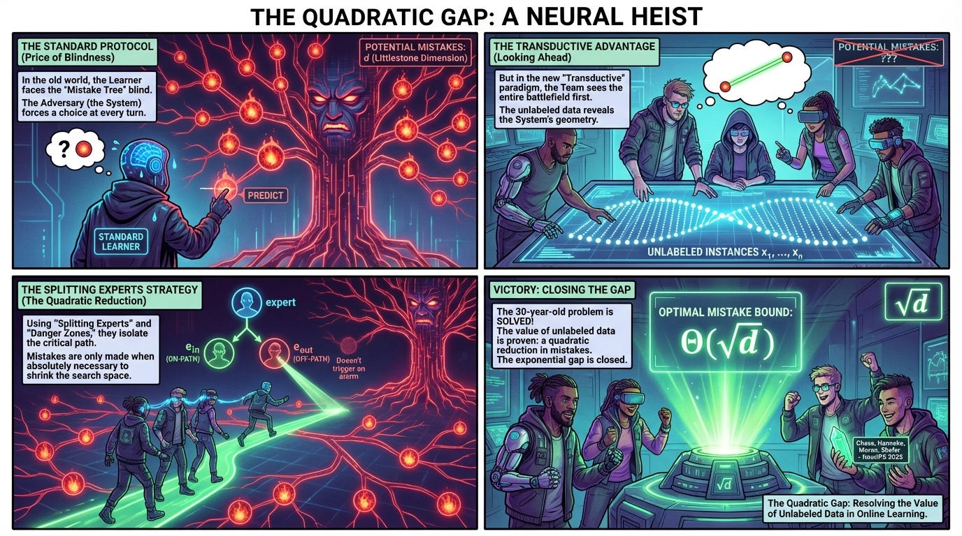
WHAT was done? The authors resolved a 30-year-old open problem in learning theory by establishing tight mistake bounds for Transductive Online Learning. Recognized as a Best Paper Runner-Up at NeurIPS 2025, they proved that for a hypothesis class with Littlestone dimension d, the optimal mistake bound is Θ(sqrt(d)).
WHY it matters? This result quantifies exactly how much “looking ahead” helps. It proves that having access to the unlabeled sequence of future test points allows for a quadratic reduction in mistakes compared to the standard online setting (where the bound is d). This closes a massive exponential gap between the previous best known lower bound of Ω(logd) and upper bound of O(d).
Details
The Information Bottleneck
The central tension in online learning theory has long been the “Price of Blindness.” In the standard online learning setting—governed by the Littlestone Dimension—the learner must predict labels sequentially without knowing what instances will arrive next. The adversary can force d mistakes by adaptively choosing the hardest path through a binary tree shattered by the hypothesis class H. However, in the Transductive Online Learning setting, the learner is granted a preview: they see the entire sequence of unlabeled instances x1,…,xn before making their first prediction. Intuitively, seeing the geometry of the data points should restrict the adversary’s ability to hide the target function.
For three decades, the magnitude of this advantage was unknown. While we knew that Transductive learning was strictly easier than Standard learning (Mtr(H)≤Mstd(H)), the bounds were loose. Prior work by Ben-David et al. (1997) established a lower bound of Ω(loglogd) (later improved to Ω(logd)) and an upper bound roughly proportional to d. This left the field wondering: is the improvement from unlabeled data exponential (like logd) or merely linear? Chase et al. settle this debate definitively: the improvement is polynomial, specifically quadratic. The optimal mistake bound is Θ(sqrt(d)).
First Principles: Trees and Sparse Encodings
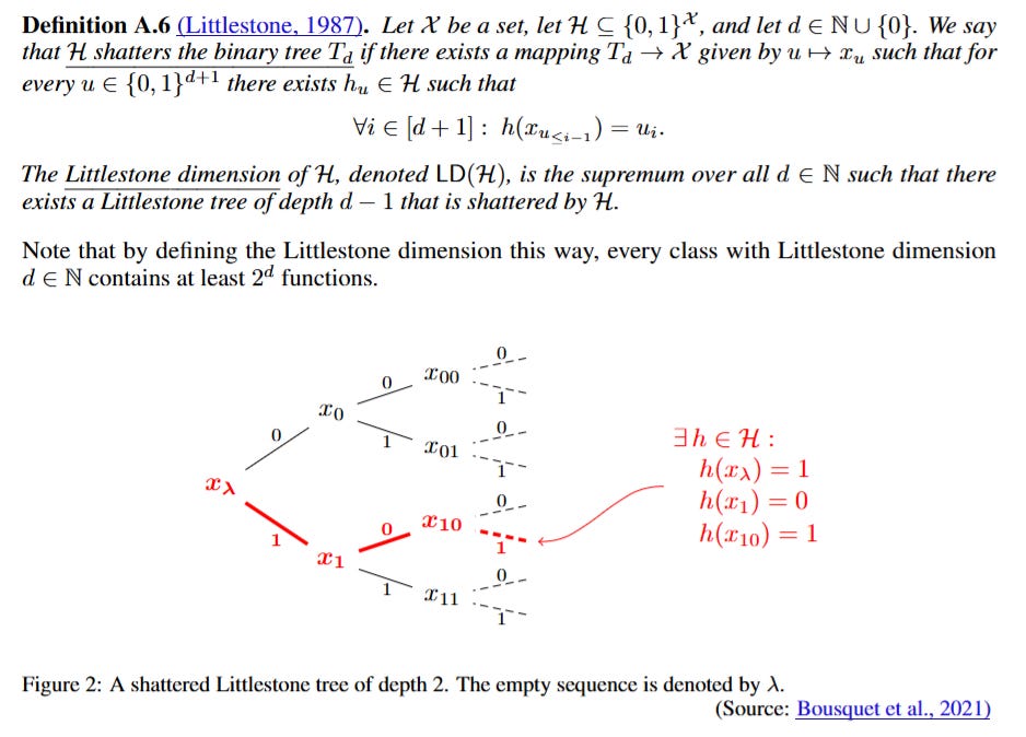
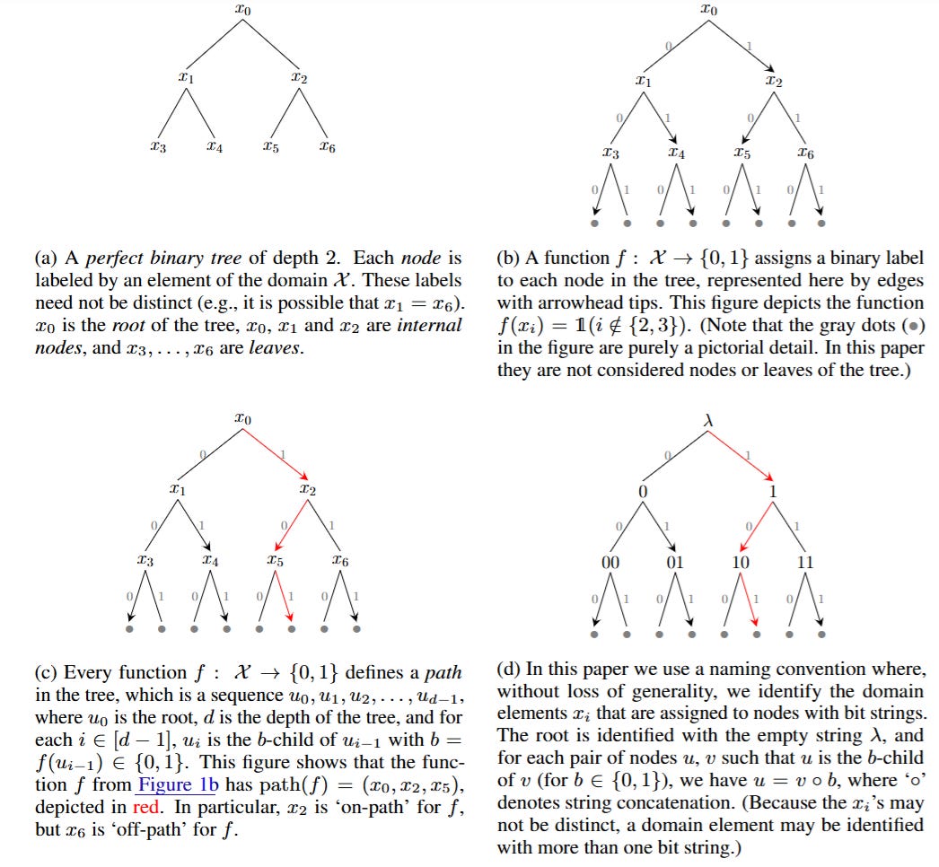
To understand the mechanics of this proof, we must revisit the atomic unit of online classification: the Littlestone Tree (Figure 1). A class H has dimension d if it can shatter a perfect binary tree of depth d. In the standard setting, the adversary forces a mistake at every node by waiting for the learner’s prediction ŷt and then setting the true label yt=1−ŷt, moving down the branch consistent with the mistake. This forces the version space (the set of viable hypotheses) to shrink, but only guarantees convergence after d steps.
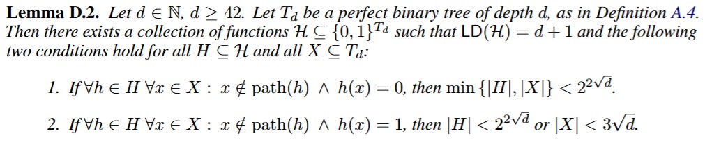
The authors’ insight relies on distinguishing between “dense” and “sparse” encodings of information. Consider the problem of guessing a number k∈{0,…,2d−1}. If encoded in binary (e.g., 1101...), the adversary can force a mistake on every bit, costing d mistakes. However, if encoded in a “one-hot” format (a string of length 2d with a single 1), a transductive learner who sees the whole string length can simply predict 0 everywhere. They will be wrong exactly once. The sequence length in the transductive setting acts as a constraint on the adversary. The paper constructs a hypothesis class (Lemma D.2) that lies in the “Goldilocks” zone between these two extremes: a class that acts like a sparse encoding (easy to guess) in the transductive setting, but retains the hard tree structure of the binary encoding in the standard setting.
The Mechanism: Danger Zones and Splitting Experts
The upper bound proof involves a novel algorithm, TRANSDUCTIVELEARNER (Algorithm 5), that exploits this sparse structure. The learner maintains a set of experts, each operating under a specific “path assumption.” When a new instance xt arrives, the learner does not know if xt is on the critical path of the target function (where the adversary has freedom to assign labels) or off-path (where labels are likely 0).
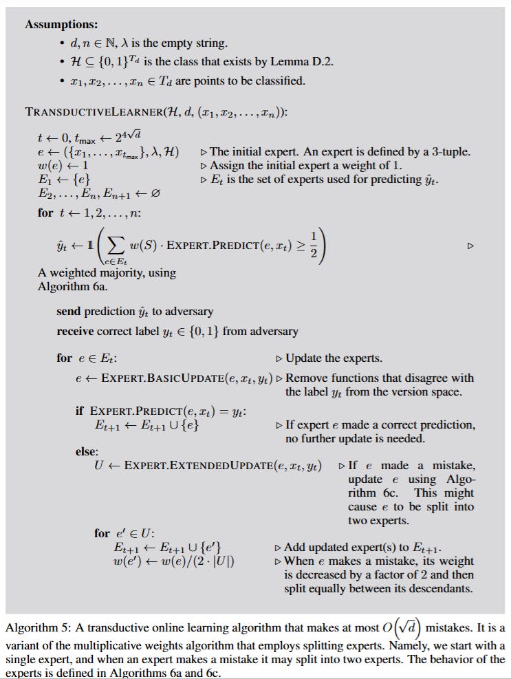
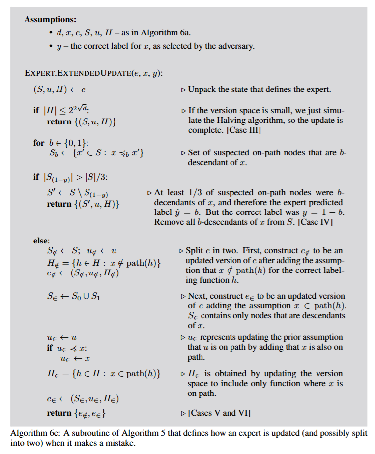
For a specific instance xt, the algorithm defines a Danger Zone, S, containing unlabeled nodes that might be on the path. The learner uses a “Splitting Experts” strategy combined with the Multiplicative Weights Update method. When an expert e encounters xt, it splits into two virtual experts via EXPERT.EXTENDEDUPDATE (Algorithm 6c): e∈ (assuming xt is on-path) and e∉ (assuming xt is off-path). If e∉ is correct (the node is off-path), the expert predicts 0. If the true label is 1 (a rare event in their sparse construction), the expert pays a mistake but the Danger Zone shrinks significantly because “off-path 1s” are highly informative. Conversely, if e∈ is correct (the node is on-path), the expert engages in a local Halving algorithm. By tuning the weights, the algorithm ensures that the total mistakes are bounded by the “best” expert, which turns out to be O(sqrt(d)). The “Danger Zone” ensures that the learner doesn’t bleed mistakes on the long sequence of irrelevant off-path nodes.
The Probabilistic Construction
To prove the matching lower bound of Ω(sqrt(d)), the authors employ the probabilistic method to demonstrate the existence of a hard hypothesis class. They do not manually build the geometry; instead, they sample a hypothesis class H where for every function h, nodes on the “true path” take values determined by the path, but nodes off-path are assigned the label 1 with a specific bias probability p=2−sqrt(d).
This specific probability p is the crux of the sqrt(d) result because it balances two competing forces. If p is too high (many 1s off-path), the learner gains too much information from the unlabeled sequence, allowing them to eliminate hypotheses too quickly. If p is too low (almost all 0s off-path), the adversary cannot punish the learner for predicting 0 on off-path nodes, making the game too easy (like the one-hot example). Setting p=2−sqrt(d) forces the adversary to use a sequence length of roughly 2sqrt(d) to confuse the learner. On this specific length, the adversary can force mistakes proportional to sqrt(d) by leveraging the “balancedness” of the version space. If the fraction of hypotheses predicting 1 is roughly 0.5, the adversary forces a mistake; otherwise, they yield to the majority, preserving the version space.
Validation and Analysis
The rigor of the paper rests on the tight coupling of the upper and lower bounds. The authors show that the sequence length n plays a critical role. They define MinLen(H, M) as the minimum sequence length required to force M mistakes. They prove that for the hard class, a sequence length of n=2Θ(sqrt(d)) is required to force d mistakes. The lower bound is explicitly demonstrated by constructing an adversary that uses a ratio rt = ∣{h∈Ht−1:h(xt)=1}∣ / ∣Ht−1∣ to guide the label generation, proving that with the probabilistic class, the adversary can maintain rt∈[ϵ,1−ϵ] for Ω(sqrt(d)) rounds. For the upper bound, the algorithm is validated by proving that at least one expert in the split ancestry correctly identifies the path nodes. The weight of this expert is lower-bounded by 2−48sqrt(d), which the Multiplicative Weights algorithm translates into a mistake bound of roughly 48sqrt(d).
Limitations
While the result is a theoretical tour de force, the practical implementation of the optimal learner is computationally prohibitive. The “Splitting Experts” strategy implies that the number of experts can grow exponentially with the number of mistakes or sequence length, as the ancestry tree branches at every ambiguity. The algorithm is an information-theoretic proof of existence rather than a lightweight method for deployment on edge devices. Furthermore, the constants in the proof (e.g., the lower bound requires d≥800) suggest that the asymptotic behavior kicks in only for highly complex hypothesis classes. The authors also leave open whether an efficient algorithm exists that runs in time polynomial in d and n, and whether the domain size must be exponential in d to achieve the bound.
Conclusion
Chase et al. have provided the definitive answer to the transductive online learning problem. By establishing the Θ(sqrt(d)) bound, they have mathematically codified the value of unlabeled data: it transforms the difficulty of learning from a linear dependence on dimension to a square root. This suggests that in realizable scenarios where test data can be batched and observed in advance (e.g., processing a fixed corpus of documents), algorithms that actively exploit the unlabeled geometry can achieve vastly superior performance guarantees than standard online approaches.