
This is how the Neocortex Learns
Authors: Randall C. O’Reilly
Paper: https://compcogneuro.org/oreilly-2026-cortlearn (https://arxiv.org/abs/2606.08720)
Code: N/A
Model: N/A
TL;DR
WHAT was done? The author presents a comprehensive, multi-level theoretical synthesis demonstrating that the mammalian neocortex learns by approximating error backpropagation. This approximation is achieved through a “temporal derivative model” where error gradients are implicitly represented as the difference between consecutive prediction and outcome activation states over a 200 ms theta cycle. The model is biologically mapped to bidirectional corticothalamic loops and implemented at the sub-cellular level through competitive kinase-driven synaptic plasticity.
WHY it matters? This work resolves a major, decades-long debate regarding the biological plausibility of deep credit assignment in the brain. By showing how the neocortex can perform gradient descent implicitly without requiring structurally segregated “error” neurons or physically impossible backward wiring, this framework provides a grand unified theory of mammalian learning. It offers a clear blueprint for the design of energy-efficient on-chip learning rules and neuromorphic architectures that can replicate the scaling properties of deep neural networks.
Details
The Credit Assignment Paradox in Biological Systems
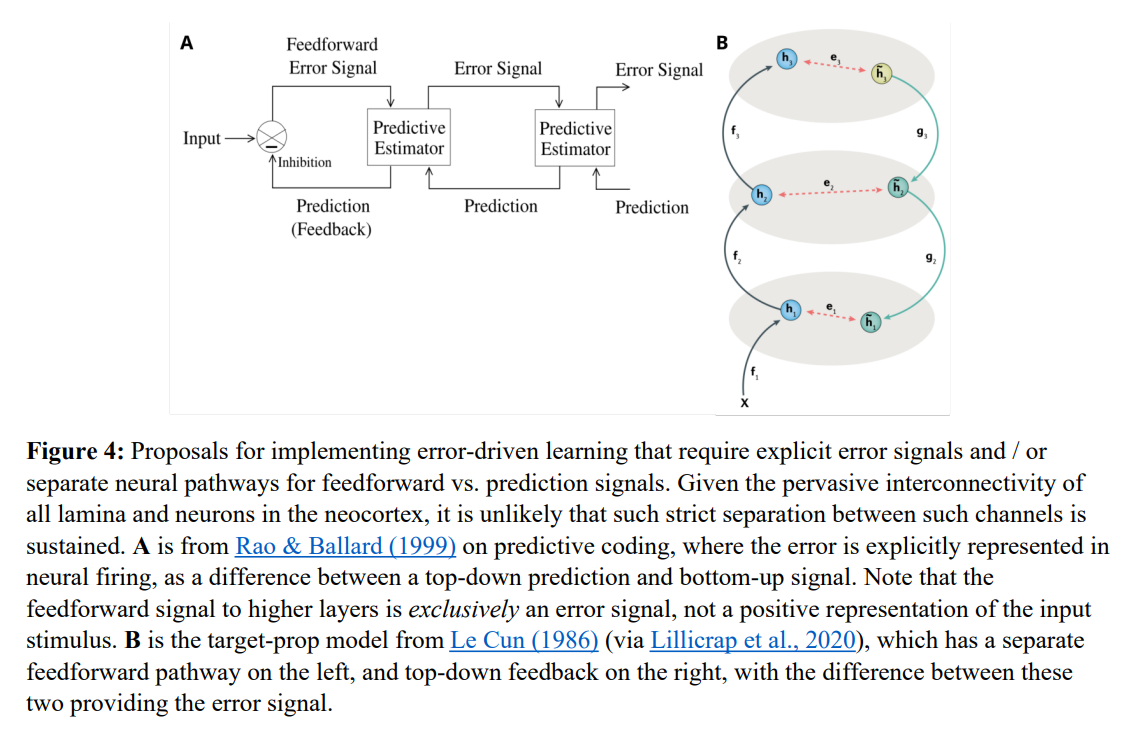
A profound tension has long existed between artificial intelligence and neurobiology. From a computational standpoint, gradient-based optimization via error backpropagation is the only mechanism demonstrated to scale to human-level representations, driving the success of modern deep networks. Yet, since early skepticism, a dominant consensus in neuroscience has held that the physical brain cannot compute these gradients (see another recent paper). Traditional models of biological learning have relied heavily on localized heuristic rules like Hebbian plasticity, which are computationally insufficient for training deep, hierarchical networks. Alternative theories attempting to bridge this gap, such as standard Predictive Coding and target-propagation, solve the credit assignment problem but introduce a different biological bottleneck. As diagrammed in Figure 4, they demand highly segregated, distinct populations of neurons to explicitly represent predictions, outcomes, and subtraction-based error signals. This represents a structural complexity that directly contradicts the highly interconnected, redundant nature of neocortical lamina.
The temporal derivative model resolves this conflict by shifting the representation of error gradients from space to time. Instead of relying on dedicated error-representing neurons, the framework proposes that the exact same cortical neurons represent both predictions and outcomes at different moments. By taking the temporal difference between these two states, the network implicitly calculates error gradients. This elegant formulation utilizes the well-established bidirectional excitatory pathways of the neocortex to perform parallel constraint satisfaction, aligning the optimization advantages of backpropagation with the biological reality of the mammalian brain.
First Principles: Formulating the Implicit Error State
To understand the mechanics of this framework, we must first define its core state variables and the mathematical approximations of the gradient. The network is conceptualized as a bidirectionally connected dynamical system. Within a given cortical area, the activation state of a neuron j undergoes a continuous evolution over a defined temporal window. Rather than explicitly computing a spatial derivative, the local error representation is approximated as the difference between two temporally distinct phases:
Error≈aj,plus−aj,minus
Here, aj,minus represents the positive, real-valued neural activation of the receiving unit j during the prediction (minus) phase, while aj,plus represents its activation during the subsequent outcome (plus) phase. Consequently, the local synaptic weight update Δwij between a sending unit i and a receiving unit j is formulated as:
Δwij∝(aj,plus−aj,minus)⋅ai,minus
In this equation, ai,minus is the sending unit’s activation during the initial prediction phase. Because all variables remain positive and compatible with standard firing rate representations, this formulation bypasses the need for negative firing rates or signed error lines. The bidirectional excitatory connections, which are highly abundant in the neocortex, allow top-down feedback from higher cortical layers to influence the activations of lower-level hidden units. This interaction ensures that the temporal difference computed locally at each synapse mathematically approximates the global backpropagated error gradient.
The Corticothalamic Loop: A Temporal Phasing Walkthrough
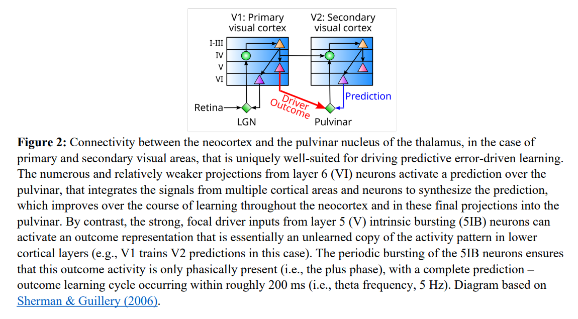
The generation and synchronization of these distinct prediction and outcome states are driven by a highly specialized anatomical architecture involving corticothalamic loops. A single learning cycle operates over a 200 ms temporal window, corresponding to the physiological theta rhythm of 5 Hz. To understand the flow of information, consider a running example of a visual stimulus processing through a primary and secondary visual area as depicted in Figure 1 and Figure 2.
During the first 100 ms, which constitutes the minus or prediction phase, a wave of bottom-up sensory input propagates from the retina through the lateral geniculate nucleus up to the cortical layers. Concurrently, numerous but relatively weak corticofugal projections from layer 6 (VI) of higher cortical areas project down to the pulvinar nucleus of the thalamus to synthesize a prediction of the expected state. Because the connections within the cortical sheet are highly bidirectional, the hidden layers and prediction layers mutually excite each other, settling into a coherent, parallel constraint-satisfaction state. At the end of this minus phase, the network’s state reflects a pure top-down prediction.
At the transition to the second 100 ms, which is the plus or outcome phase, the actual sensory outcome is presented. This state change is driven by a small number of abnormally strong, focal “driver” inputs originating from layer 5b intrinsic bursting (5IB) neurons of hierarchically lower areas, which burst periodically at the theta frequency. As shown in Figure 2, these powerful bursting drivers override the weak layer 6 predictive inputs at the level of the pulvinar, instating a high-fidelity representation of the actual outcome. This updated state is then projected top-down via thalamocortical relay cells back to the neocortex. This dual-phase sequence forces the entire neocortical hierarchy to transition from a predictive state to an outcome-driven state, establishing the temporal difference required for local gradient computation.
Molecular Computation: Competitive Kinase Integrators
Descending to the implementational level, the model explains how individual synapses physically compute the difference between these fast-moving temporal phases. The physical calculation is achieved through a competitive, double-kinase intracellular signaling pathway. Locally at the post-synaptic density, the temporal derivative is computed as the difference between a fast and a slow integral of calcium-activated calmodulin (CaM). The dynamics of these leaky integration channels are governed by first-order differential equations driven by the intracellular calcium concentration Ca(t), which acts as a biochemical proxy for neural activity:
In these equations, Ifast(t) represents the fast-integrating signal that tracks the transient calcium influx of the immediate outcome (plus) phase, while Islow(t) represents the slower integrator that filters out high-frequency fluctuations to retain a biochemical trace of the earlier prediction (minus) phase. The respective integration time constants satisfy the inequality τfast≪τslow. The local synaptic weight change Δw is then dictated by the difference between these two integration signals at the end of the theta cycle:
Δw∝Ifast−Islow
This mathematical integration is directly mapped to the competitive dynamics of two enzymes: calcium/calmodulin-dependent protein kinase II (CaMKII) and death-associated protein kinase 1 (DAPK1). If CaMKII possesses a faster activation and integration rate in response to the common calcium-calmodulin driver, it will dominate during positive temporal derivatives, driving Long-Term Potentiation (LTP). Conversely, if DAPK1 integrates the signal more slowly, it will dominate when the temporal derivative is negative, leading to Long-Term Depression (LTD). This competitive molecular switch allows individual physical synapses to calculate error derivatives locally, without requiring global orchestration.
Empirical Disruption of Hebbian Dogma
The validity of this kinase-driven temporal derivative model is strongly supported by recent in vitro synaptic plasticity experiments. Pyramidal neurons were stimulated with highly controlled temporal patterns of activity over a 200 ms window to emulate the prediction and outcome phases, with the results summarized in Figure 3.
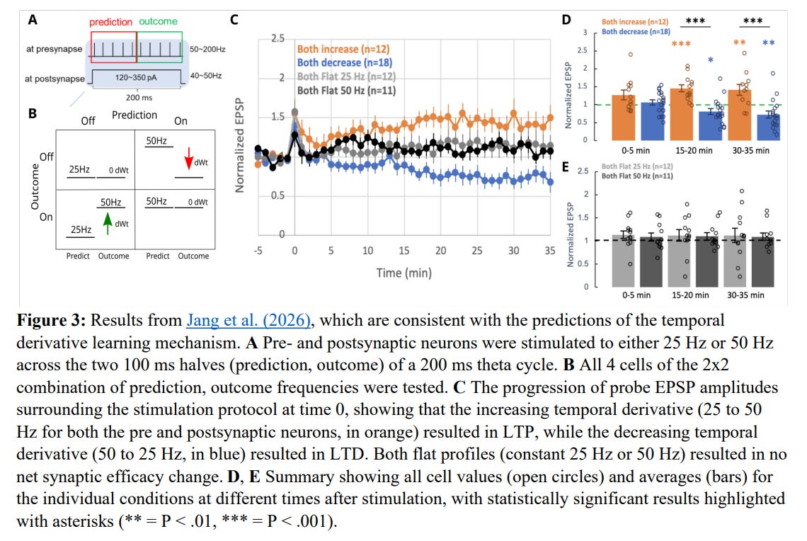
When the stimulation frequency rose from a 25 Hz prediction phase to a 50 Hz outcome phase, a strong positive temporal derivative was created, resulting in significant LTP where the normalized excitatory postsynaptic potential (EPSP) amplitude rose to approximately 1.5 to 1.8. Conversely, when the pattern was reversed from 50 Hz down to 25 Hz, creating a negative temporal derivative, LTD was observed, with the EPSP dropping to approximately 0.8. Crucially, flat stimulation profiles of constant 25 Hz or constant 50 Hz resulted in absolutely no net change in synaptic efficacy.
These findings directly challenge classical Hebbian learning models, such as those governed by the BCM theory. Under standard Hebbian assumptions, high-frequency co-activity (such as the 50-50 Hz condition) should yield the strongest calcium influx and thus the maximum possible LTP. The observation that a 50-50 Hz flat profile results in zero net plasticity, whereas a 25-50 Hz profile with lower net activity drives robust LTP, proves that the synapse is sensitive to the temporal derivative of activity rather than its absolute magnitude.
Genealogy of Phase-Based Backpropagation
The temporal derivative framework is not an isolated development; it represents the culmination of a rich lineage of phase-based learning algorithms. The core concept of utilizing distinct phases of neural activity to compute error gradients was pioneered with the Boltzmann Machine (Ackley et al., 1985), which utilized a contrastive learning rule based on “clamped” and “unclamped” states. This mathematical foundation was subsequently brought closer to backpropagation through the Recirculation model (Hinton & McClelland, 1988) and its generalized successor, the GeneRec algorithm (O’Reilly, 1996), which explicitly derived backpropagation-approximating gradients from local temporal differences.
More recently, this lineage has expanded to include Equilibrium Propagation (Scellier & Bengio, 2017), which shares a similar mathematical structure but relies on continuous energy minimization. The temporal derivative model proposed here distinguishes itself from these ancestors by directly mapping these abstract mathematical phases onto specific, well-characterized biological substrates, such as the 200 ms thalamocortical theta rhythm and molecular kinase switches. It also functions alongside specialized auxiliary systems, such as Behavioral Timescale Synaptic Plasticity (Magee, 2026), which acts as a rapid-mapping system to quickly decode the slowly-accumulating statistical representations constructed by deep corticothalamic credit assignment.

Unresolved Nodes and Scaling Friction
Despite its theoretical elegance, several critical challenges remain before the temporal derivative model can be accepted as a complete account of neocortical learning. At the structural level, while the model details the role of pulvinar projections, the precise driving target signals that guide the plasticity of layer 5 neocortical output neurons remain partially unresolved. The current hypothesis relies heavily on broad, matrix-type thalamic projections from the ventral anterior nucleus, but detailed experimental mapping is required to confirm this pathway.
Furthermore, the empirical foundation of the model relies on very recent, highly specialized in vitro synaptic preparations. These findings must be replicated across different cortical regions and in vivo preparations to prove that the 200 ms theta-frequency temporal phasing is a universal computational principle of the neocortex. Finally, from an engineering perspective, although the model has been implemented in spiking neural networks within the WebGPU-accelerated Axon framework, it has yet to be demonstrated that this local, phase-based learning can scale to match the performance of standard backpropagation on massive, modern deep learning benchmarks.
Strategic Synthesis and Neuromorphic Horizons
The strategic value of this paper lies in its rigorous execution of Marr’s tri-level vision, successfully linking abstract computational requirements to concrete biological machinery. By demonstrating that the neocortex can approximate the mathematical gradient of backpropagation without violating biological constraints, the paper dismantles the historic division between artificial and biological neural systems.

For the AI and neuromorphic hardware communities, this framework is highly significant. It provides a mathematically sound, localized learning rule that eliminates the memory-intensive global backward pass required by traditional deep learning. Implementing this competitive kinase-based temporal difference rule in analog silicon or spiking hardware could enable ultra-low-power, on-chip, continuous learning agents. Ultimately, this work offers a highly compelling working hypothesis for neocortical learning, suggesting that the most powerful algorithm of artificial intelligence is, in fact, the very mechanism that drives human cognition.