
Authors: David Klindt, Yann LeCun, Randall Balestriero
Paper: https://arxiv.org/abs/2605.26379v1
Code: https://github.com/klindtlab/lejepa-identifiability
Model: N/A
TL;DR
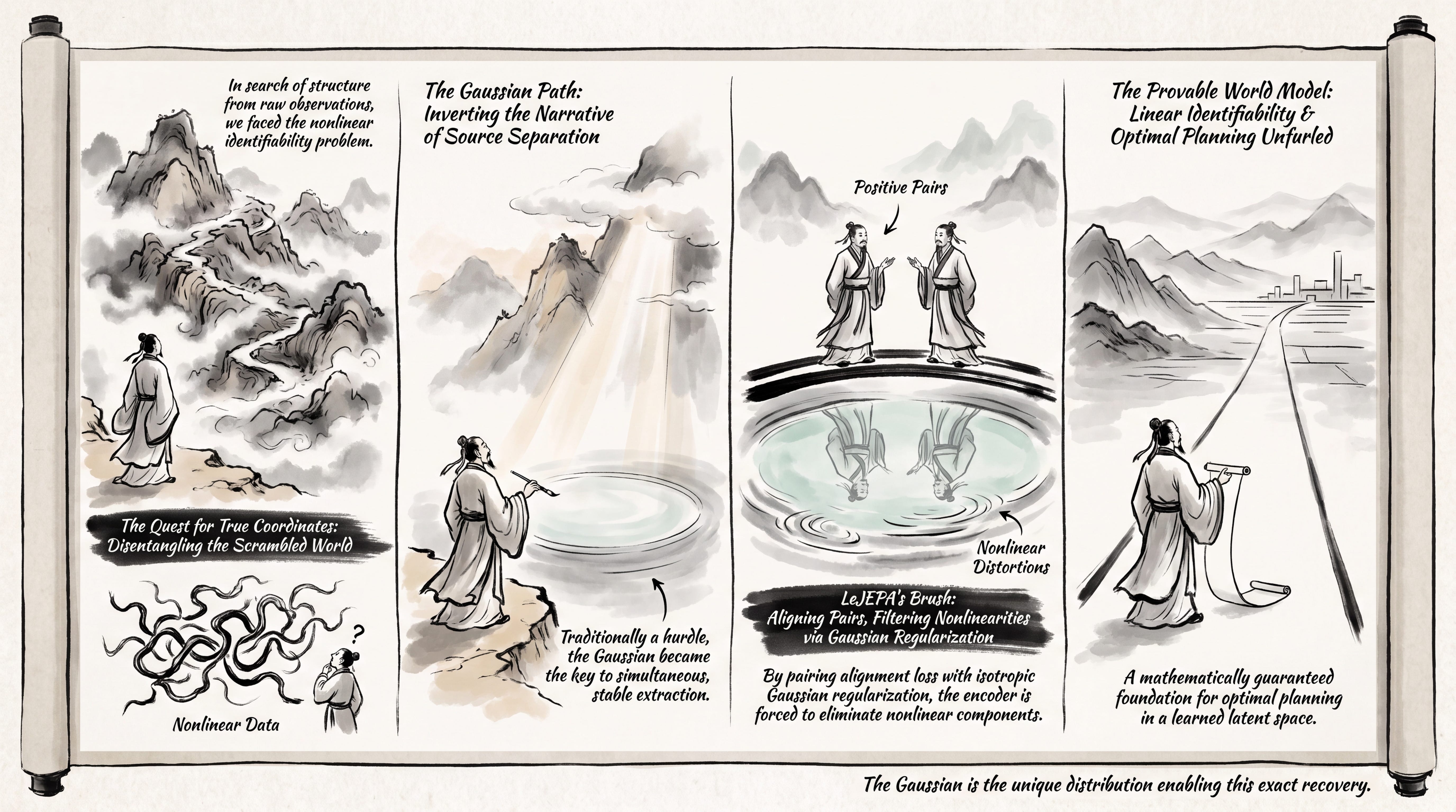
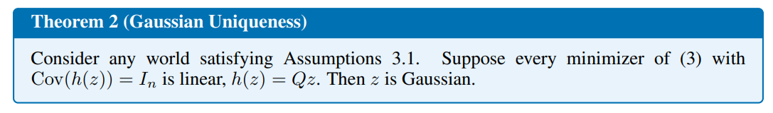
WHAT was done? The authors present the first formal mathematical proof of linear identifiability for Joint-Embedding Predictive Architectures (JEPAs). They prove that LeJEPA [review] (which pairs an alignment loss with isotropic Gaussian regularization) linearly recovers a generative world’s true latent variables from complex, nonlinear observations up to an orthogonal rotation. Crucially, they establish that within a broad class of stationary, additive-noise environments, the Gaussian is the unique distribution that guarantees this exact recovery.
WHY it matters? In nonlinear representation learning and unsupervised representation learning (Nonlinear ICA), the Gaussian has historically been viewed as the single distribution where source separation fails. This work inverts that narrative, proving that the Gaussian is precisely what enables simultaneous, stable extraction of all latent dimensions at scale. Furthermore, the authors prove that this linear, orthogonal identifiability is theoretically sufficient to enable optimal planning directly in the learned latent space, offering a rigorous theoretical foundation for constructing provably correct World Models for robotics and reinforcement learning.
Details
The Quest for Identifiable Representations in Joint-Embedding Architectures
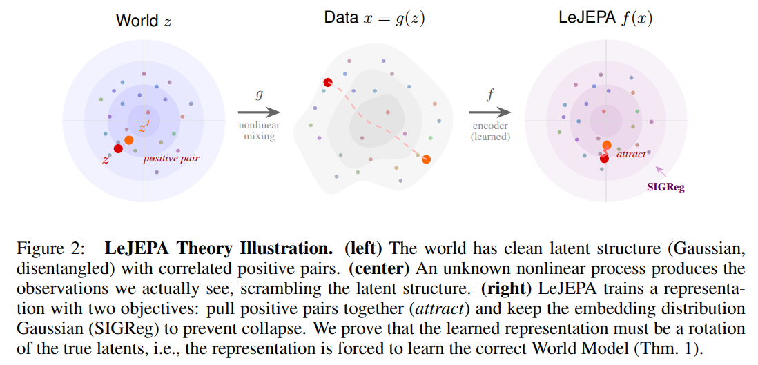
A central goal of self-supervised learning is to build world models that extract clean, disentangled, and structured representations from raw, high-dimensional observations without any manual labeling. Joint-Embedding Predictive Architectures, such as LeJEPA [review] or LeWorldModel [review], address this by training encoders to produce highly similar embeddings for temporally or spatially related views of the same underlying content. While these models have seen immense empirical success, we have historically lacked mathematical guarantees that the learned coordinates correspond to the physical degrees of freedom of the world. This represents a major theoretical bottleneck: if an encoder scrambles or entangles independent variables, downstream planners will fail to generalize when the environment undergoes basic shifts.
The primary contribution of this work is resolving this bottleneck by demonstrating that JEPAs can provide linear identifiability—a guarantee that the representation is a linear function of the true latents up to simple symmetries. This differs drastically from traditional nonlinear Independent Component Analysis (ICA) frameworks, which typically restrict representations to smooth, invertible coordinate transformations (diffeomorphisms) and are highly sensitive to optimization instabilities. By leveraging LeJEPA’s explicit Gaussian regularization (SIGReg), this research proves that we can simultaneously identify all latent factors, providing the first formal proof of representation recovery for joint-embedding methods.
Mathematical Foundations: The Generative World and the Ornstein-Uhlenbeck Channel
To establish this guarantee, the authors formulate a rigorous description of both the data-generating process and the learner’s objectives. They define the world using a set of independent, stationary latent variables z∈Rn, which are rendered into high-dimensional observations x∈Rd through an unknown, highly nonlinear mapping x=g(z).
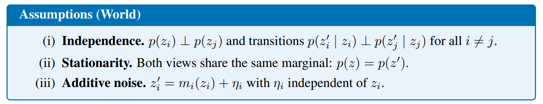
The learner trains an encoder f:Rd→Rn to produce representations, yielding a composed mapping h=f∘g from the true latent space back to the representation space. The positive pairs of observations correspond to consecutive states in the world, which are modeled using the Ornstein-Uhlenbeck (OU) transition process: z′=ρz+sqrt(1−ρ2)η In this transition rule, z represents the initial state, z′ represents the consecutive positive view, ρ∈(0,1) acts as a temporal autocorrelation parameter dictating step size, and η∼N(0,In) represents independent Gaussian transition noise orthogonal to z. Under these assumptions, the stationary distribution of the latents is an isotropic Gaussian, z∼N(0,In), which matches the maximum-entropy distribution for a fixed mean and variance.
The learner optimizes the composed representation h(z) using a combination of an alignment loss that pulls positive pairs together and a Gaussianity constraint to prevent representation collapse:
Here, the objective function L(h) measures the mean squared distance between the embeddings of related views, while the constraint forces the marginal distribution of the learned representations to follow a standard isotropic Gaussian.
Spectral Decomposition and the Inversion of Nonlinearities via Hermite Polynomials
The core mechanism behind the linear identifiability proof rests on the spectral decomposition of the world’s transition operator. For any scalar-valued function hi(z), the transition operator T computes its expected value at the next step given its current state: (Thi)(z)=E[hi(z′)∣z]. In a Gaussian world, the eigenfunctions of this operator are the probabilist’s Hermite polynomials {Hek}k≥0, which form an orthonormal basis for functions under a Gaussian measure. For a univariate variable x, these are defined sequentially starting with He1(x)=x for the linear term and He2(x)=x2−1 for the quadratic term.
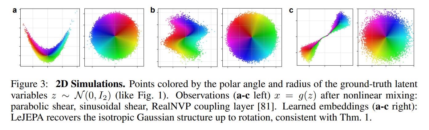
To understand how the system recovers the true coordinates, consider a specific 2D running example where the true independent latents are scrambled into a spiral observation space x=g(z) (as illustrated in the transition from left to center in Figure 1). The encoder f(x) must map this spiral back to a flat isotropic Gaussian space. Using Mehler’s formula, the eigenvalue of a degree-d Hermite polynomial is exactly ρd. Because the correlation parameter satisfies ρ∈(0,1), it follows that ρ>ρ2>ρ3>…, meaning that any nonlinear contribution (where d≥2) geometrically attenuates the temporal correlation between positive views.
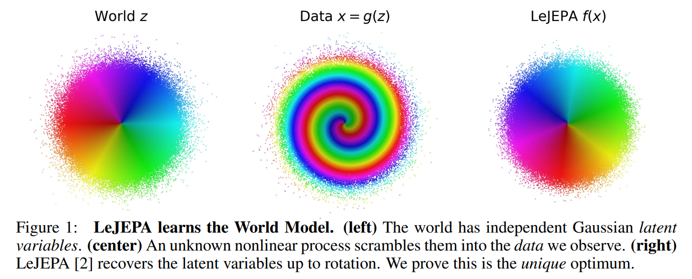
Therefore, any nonlinear distortion of the representation strictly increases the alignment loss L(h). At the global optimum, the encoder is mathematically forced to eliminate all nonlinear components of the mapping. The only representations that can satisfy the Gaussianity constraint while achieving maximum correlation are purely linear combinations of the first-degree Hermite polynomials, which correspond to the raw coordinate functions themselves. Thus, the optimal representation satisfies h(z)=Qz for an orthogonal rotation matrix Q∈O(n), successfully unmixing the nonlinear observation back to its true latent coordinates (as shown qualitatively in Figure 3).
Scaling up to High-Dimensional Spaces and Optimization Dynamics
To translate these theoretical population-level statements into scalable algorithms, the authors optimize a balanced objective combining the empirical invariance (alignment) loss Linv and Sketched Isotropic Gaussian Regularization (SIGReg) LSIG:L=λLSIG+(1−λ)Linv In this practical objective, λ∈[0,1] is a balancing coefficient that controls the relative weight of the Gaussian regularization.
For controlled 2D settings, the authors parameterized the encoder f as a 4-layer Multi-Layer Perceptron (MLP) with a hidden dimension of 256 and GELU activation functions. To evaluate the framework’s scalability, they conducted dimensional sweeps up to N=1024 latent dimensions using a matched RealNVP-style inverse coupling layer architecture with tanh activations. For high-dimensional, raw-pixel inputs, they utilized a deep Convolutional Neural Network (CNN) containing BatchNorm layers and approximately 1.1 million parameters, as detailed in Section H.11.
The training relied on the AdamW optimizer with a learning rate of 3×10⁻³, utilizing a 10,000-step linear warmup followed by a 10,000-step cosine decay schedule. Applying gradient clipping with a maximum norm threshold of ∥∇∥max=1.0 proved essential for preventing instabilities. Empirically, the inclusion of BatchNorm was critical for stabilizing the representation; omitting it caused 36% of the CNN runs to collapse to zero-variance.
Empirical Robustness and the Verification of Approximate Identifiability
In practical applications, exact alignment and perfect whitening are never fully achieved, necessitating an understanding of how the model behaves under approximation errors. To address this, the authors formulated Theorem 3, which establishes a robust stability bound: E[∥h(z)−Qz∥2]≤D+(ε+D)2 Here, ε=∥Cov(h(z))−In∥F represents the covariance deviation from a perfectly whitened identity matrix, while D=δ/(2ρ(1−ρ)) represents the normalized alignment gap. The term δ=L(h)−2(1−ρ)tr(Cov(h(z))) captures the excess loss above the optimal linear alignment limit.
This bound was empirically verified through extensive grid searches across varying values of the regularization weight λ and autocorrelation ρ, as shown in Figure 4a and Figure 9.
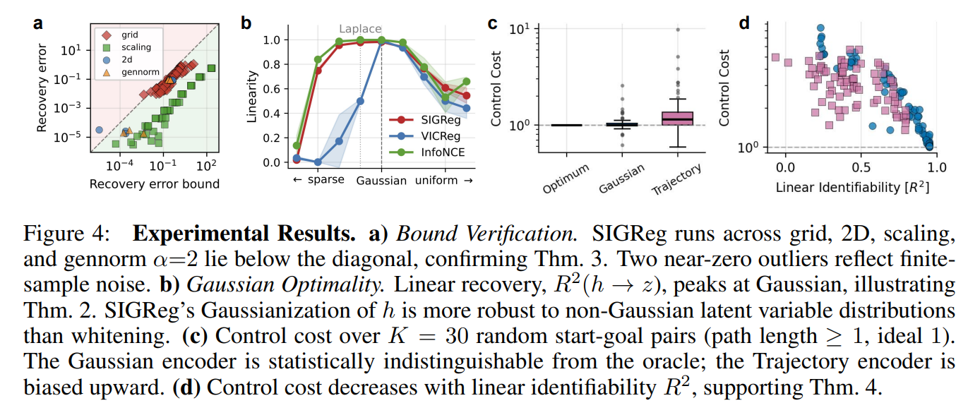
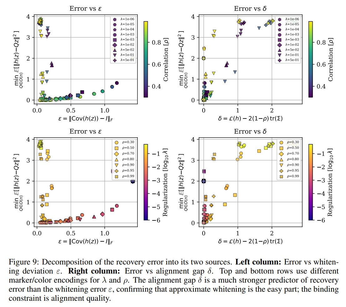
The experiments demonstrate that the alignment gap δ is the primary predictor of overall representation recovery error, indicating that approximate whitening is relatively easy to satisfy in practice, whereas the quality of the alignment objective remains the binding constraint.
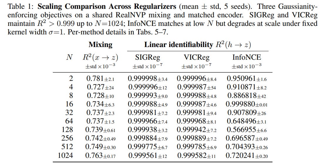
The dimensional scaling experiments summarized in Table 1 reveal a stark contrast between different self-supervised baselines. Both SIGReg (LeJEPA) and VICReg maintain near-perfect linear recovery (R2>0.999) up to N=1024 dimensions. Conversely, InfoNCE suffers from severe performance degradation at high dimensions, with its R2 dropping to approximately 0.72 at 1024 dimensions due to Gaussian kernel underflow under a fixed kernel width.
Connecting JEPAs to Nonlinear ICA and Slow Feature Analysis
This theoretical framework shares deep connections with Slow Feature Analysis (SFA) and classical Nonlinear ICA. SFA objectives also seek functions that vary as slowly as possible over time, which mathematically aligns with JEPAs’ goal of maximizing temporal correlation. However, classical SFA implementations rely on fragile, sequential, and greedy extraction techniques that project out nonlinear transformations step-by-step. This sequential pipeline accumulates estimation errors rapidly and degrades when scaled beyond a few dimensions.
By contrast, JEPAs solve this problem by simultaneously optimizing all representation dimensions through a joint loss containing a multidimensional whitening or Gaussianity constraint. Because whitening is invariant under orthogonal rotations, this joint optimization yields an orthogonal identifiability class, which is far more stable at scale. Furthermore, whereas classical linear ICA models fail to identify independent sources when they are Gaussian, this nonlinear setup demonstrates that the Gaussian distribution is the unique catalyst that enables clean, linear source separation under stationary transitions.
Theoretical Boundaries: Gaussian Assumptions and Dimensional Mismatches
Despite the elegance of the proofs, several critical limitations must be highlighted. First, the uniqueness guarantee (Theorem 2) relies heavily on the assumption that the world’s latent variables are Gaussian.
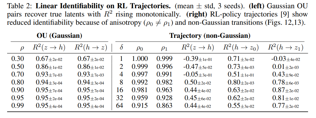
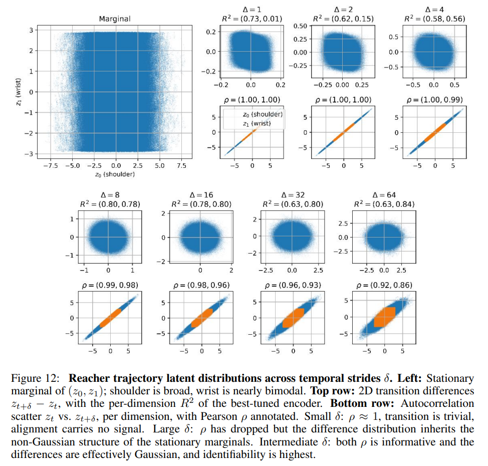
When this assumption is violated, linear identifiability can degrade. This degradation is clearly visible in the pixel-based DeepMind Control Suite Reacher trajectory task (Table 2 and Figure 12), where the joint-angle distributions of a goal-directed policy exhibit highly non-Gaussian, anisotropic properties. Under these conditions, the total recovery R2 drops below 0.5, indicating that the encoder begins recovering higher-order, nonlinear Hermite polynomials instead of the true linear coordinates.
Second, the proof assumes that the encoder’s output dimension exactly matches the true latent dimension (m=n). If the encoder has excess capacity (m>n), the system may experience redundant coordinate encoding, whereas insufficient capacity (m<n) can result in representation collapse or superposition. Finally, the theoretical guarantees represent population-level statements about global optima, leaving the finite-sample scaling laws and detailed training dynamics of the gradient descent path as open questions for future research.
The Strategic Verdict: A Mathematically Provable Foundation for World Models
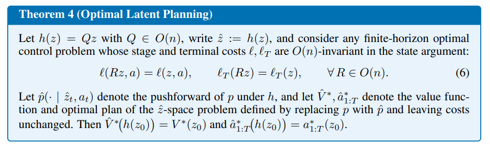
The ultimate value of this work lies in Theorem 4, which demonstrates that linear, orthogonal identifiability is theoretically sufficient to enable optimal planning directly in the learned representation space. Under an orthogonally invariant cost function—such as goal-reaching costs measuring Euclidean distance—the trajectories planned in the learned latent space are mathematically identical to those planned in the true physical state space.
As qualitatively verified in the robotic planning visualization (Figure 5 and Figure 17), a planner utilizing a Gaussian-regularized encoder successfully recovers straight-line paths in the physical joint space, while a non-Gaussian trajectory encoder produces highly distorted, energetically inefficient paths.

This means that classical control algorithms (such as the Linear-Quadratic Regulator) can be integrated directly with self-supervised visual encoders without requiring complex, manual calibration of the coordinate systems. For researchers and engineers building autonomous systems, this paper provides a robust, provably correct foundation for designing and scaling future World Models.